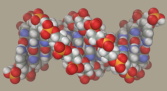
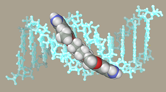
DNA-ligand modeling

Let us generate a DNA model with a ligand in the minor groove.

DNA

Open the Chain Editor . Select the B-DNA section and enter a DNA sequence. For instance, enter the classical sequence CGCGAATTCGCG into the lower Sequence window and press the Apply button. A DNA model with a conformation close to the Arnott’s conformation is displayed. Save it to a file.

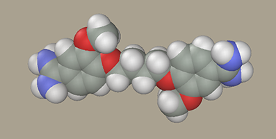
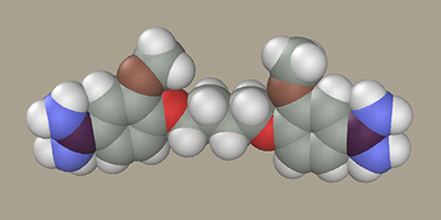
Ligand

Select the Chain Editor B-DNA ligands section. Several residue samples are available there to construct ligands of the pentamidine series (J Med Chem, 1992, v. 35, pp.431-438) as well as residues to construct the alkyl bridge. For example, select AmPh(OMe)OCH2- L and click -CH2- twice and AmPh(OMe)OCH2- R once. Note that two -CH2- were selected, while the resulting model has four methylene groups. The point is that the methylene groups attached to oxygen have partial atomic charges different from those in carbohydrates. Accordingly, such methylene groups were added to the model of the ligand terminal residue (AmPh(OMe)OCH2-) in advance.

Rotate the ligand OMe groups so that they face the same direction. This can be done by a short molecular dynamics simulation with restraints imposed on the model. The molecule should remain extended and the OMe groups should face the same direction. Invoke the Geometry Editor .

1. Click the terminal (amidine) carbon atoms. One can see that the distance between them is 16.92 Å. Click the Fix button to accept this distance as equilibrium for the restraint imposed. Now click the Restrain button to impose the restraint with R_eqv=16.92 Å and K_R=5 kcal/mol Å. The atoms to which the restraint was applied become selected to indicate that the operation has been completed.
2. Click the oxygen atoms of the OMe groups. The distance between them is 11.4 Å. Set R_eqv equal to 9 Å and impose one more restraint (with the Restrain button). This restraint brings the OMe groups together and, hence, orients them in the same direction.

Invoke the Molecular Dynamics panel , set the temperature to 50 K and start the simulation. After some time, the molecule acquires the desired conformation. Stop the simulation and save the model to disk.

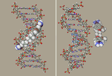
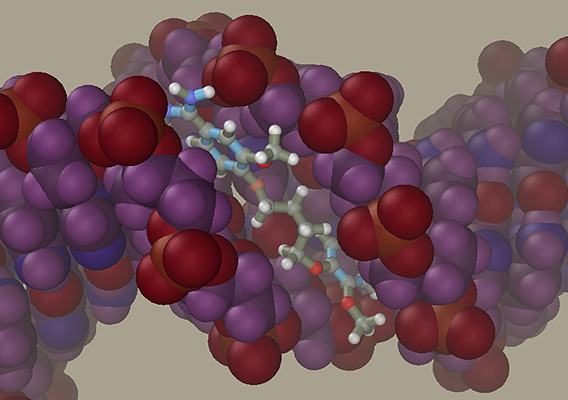
DNA-Ligand Complex

Now add the DNA model generated previously to the ligand model. Select the Add command in the File menu. At this moment, the initial and added models can be moved relative to each other, but we will not do it and press the OK button. Our ligand model has several selected atoms (if not, at least one of them should be selected with the right mouse). The molecules containing at least one selected atom can be moved relative to the rest of the model using a mouse with both buttons depressed. Place the ligand in front of the central part of DNA to face the minor groove using the Ctrl and Shift buttons and mouse. Avoid introducing the ligand directly into the minor groove, since this will cause strong collisions between atoms. Instead, place the ligand at some distance and use restraints to get it in desired place. Imagine that you attach rubber bands to the ligand and DNA, after which they contract and drive the ligand into the groove.

DNA is a relatively flexible construction. It can be deformed if the ligand runs into it at high speed. To avoid it, freeze DNA to allow movement of ligand atoms only.

• Press Esc to cancel current selection.
• Select a ligand atom.
• Select Expand to molecule in the Select menu to select the ligand molecule.
• Double-click the right mouse button to invert the selection. Now DNA is selected.
• Press the Freeze atom movement button. DNA becomes light blue to show that this part of the molecule is frozen and will not move during simulation.

Using the Geometry panel , impose restraints between the ligand and DNA and start the dynamics. After some time, the ligand is retracted into the minor groove. Impose and release restraints (Edit > Delete restraints menu) to make the ligand take the desired position. The restraints can be imposed and released without stopping the molecular dynamics.

The calculation can be accelerated by minimizing the window with the model, since showing the movement takes much processor time.

After the preliminary optimization, the simulation can be started with no restrains or frozen molecules. The molecular dynamics in vacuum is practicable at low temperatures only, since normal temperature can destroy such crude models. Such molecular dynamics is an optimization approach to generate and roughly evaluate a model. Models with explicit solvents are recommended for simulations under normal conditions.